CARTO BigQuery Tiler is a solution to visualize very large spatial datasets from BigQuery.
If you have small datasets (few megabytes) on BigQuery you can use available solutions like GeoVizQuery or CARTOframes to visualize them, but if you have millions, or even billions, of rows, you need a system to load them progressively on a map. CARTO BigQuery Tiler allows you to do that without having to move your data out of BigQuery.
CARTO BigQuery Tiler is:
- Convenient: You can run it through our UI or directly as SQL commands in BigQuery. The data never leaves BigQuery so you don't have to worry about security and additional ETLs.
- Fast: CARTO BigQuery Tiler benefits from the massive scalability capabilities of BigQuery and can process hundreds of millions of rows in a few minutes.
- Scalable: This solution works for 1M points or 100B points.
- Cost-effective: Since BigQuery separates storage from computing, the actual cost of hosting these Tilesets is very low. Additionally since you run the tiling on demand you only pay for that processing and you don't need to have a cluster available. Finally, thanks to our partitioning technology, serving tiles is very cost effective.
This project is currently only available in a private BETA. Upon request, we will grant you access to the UDF functions necessary to generate and visualize tilesets. Since permissions are associated with your BigQuery username, we'll need your Google Cloud email.
You can request access by filling out the form at https://carto.com/bigquery/beta/. Also, please consider subscribing to the beta mailing list to ask any questions, report any issues or provide feedback. Thanks.
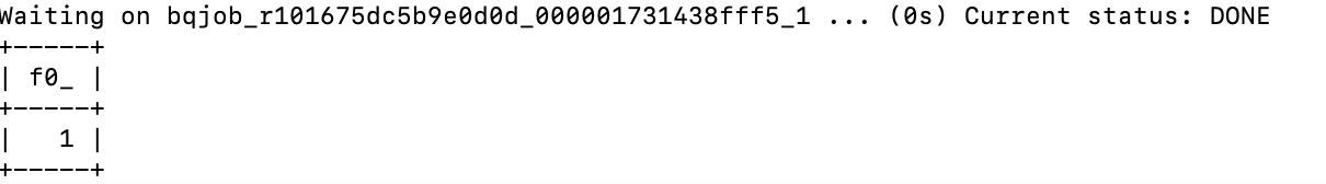
To confirm that you have access try running this query on the console:
SELECT cartobq.tiler.Version()You should get a numeric response when everything is in order. If you get a permission error that means you still don't have access and will have to contact us.
This project provides 3 components:
- A series of UDF functions and procedures for converting a spatial dataset into a tileset, that is a table that contains vector tiles (MVT) that many visualization libraries
- A CLI tool to upload, download and view generated tilesets privately.
- A WebUI to access public tilesets that you have created.
You use the UDF functions to process a dataset and generate a new table containing the vector tiles, a tileset. Then you can either use the CLI tool to visualize the tileset privately, or you can make the map public and use a WebUI to serve the map tiles.
There are 2 main procedures you can use to tilify a dataset, depending on what kind of visualization you need:
CreatePointAggregationTileset:
- You have a point dataset (or something that can be converted to points) and you want to see it aggregated.
- The points will be aggregated into cells. Each feature or cell represents all the points that fall under it, so the associated properties available for visualization are generated by aggregating the values in the source dataset.
- Values of individual points are available using single_point_properties which will only be included when a cell includes only one point. Remember that you could also get similar values with the aggregated properties using functions like ANY_VALUE or FIRST_VALUE.
CreateSimpleTileset:
- You have a dataset with any geography type (point, line or polygon) and you want to see it at an appropriate zoom level.
- The geographies will be represented exactly as stored in BigQuery, which means that if they are too small to be visible at a certain zoom level they won't be included as part of that zoom level.
- The values associated with each feature are exactly the same as the ones available in the source dataset.
Let's see a couple of quick examples on how the process works.
NYC trees (CreatePointAggregationTileset)
We are going to visualize an aggregation of the trees in New York. For each cell, we want to know how many trees are on it, so we add a new property, aggregated_total to the data. In yellow we specify the source query and in green the name of the target table that will contain the tileset.
With the query ready, you can open your BigQuery console and run it after replacing the target table name.
CALL cartobq.tiler.CreatePointAggregationTileset(
--SQL to use as the source (uses geom as the name for the geography)
'''(SELECT ST_GEOGPOINT(longitude, latitude) as geom, * FROM `bigquery-public-data.new_york_trees.tree_census_2015`)''',

--Name and location where the Tileset will be stored.
--Replace MYORGANIZATIONNAME.maps.nyc_tress_tileset with
--YOUR destination where to store the Tileset.
  '`MYORGANIZATIONNAME.MYDATASETID.nyc_trees_tileset`',

--Options on how to generate the Tileset
  '''{
      "zoom_max": 14,
      "type": "quadkey",
      "resolution": 8,
      "placement": "features-centroid",
      "properties":{
        "aggregated_total": {
          "formula": "count(*)",
          "type": "Number"
        }
      },
      "single_point_properties": {
           "tree_id": "Number",
           "address": "String"
      }
 }''');
Making the tileset public
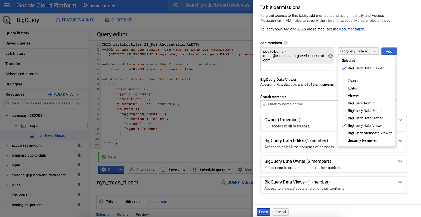
Now that we have generated the tileset we are going to make it public so we can publish and share it. For that we have to give permissions (BigQuery Data Viewer) to the table `MYORGANIZATIONNAME.MYDATASETID.nyc_trees_tileset`. There are different options:
- Make the tileset available to anyone in the internet using the
allUsersmember - Make the tileset available to anyone authenticated with a Google account using the
allAuthenticatedUsersmember - Make the tileset available only to CARTO Maps API v2 beta Service Account:
maps-api-v2@avid-wavelet-844.iam.gserviceaccount.com
Visualizing the tileset in a web browser
Once you have published the tileset, you can visualize it using a viewer accessible in the following URL::
https://viewer.carto.com/user/YOURCARTOUSERNAME/bigquery?data=ORGANIZATIONNAME.DATASETID.nyc_trees_tileset
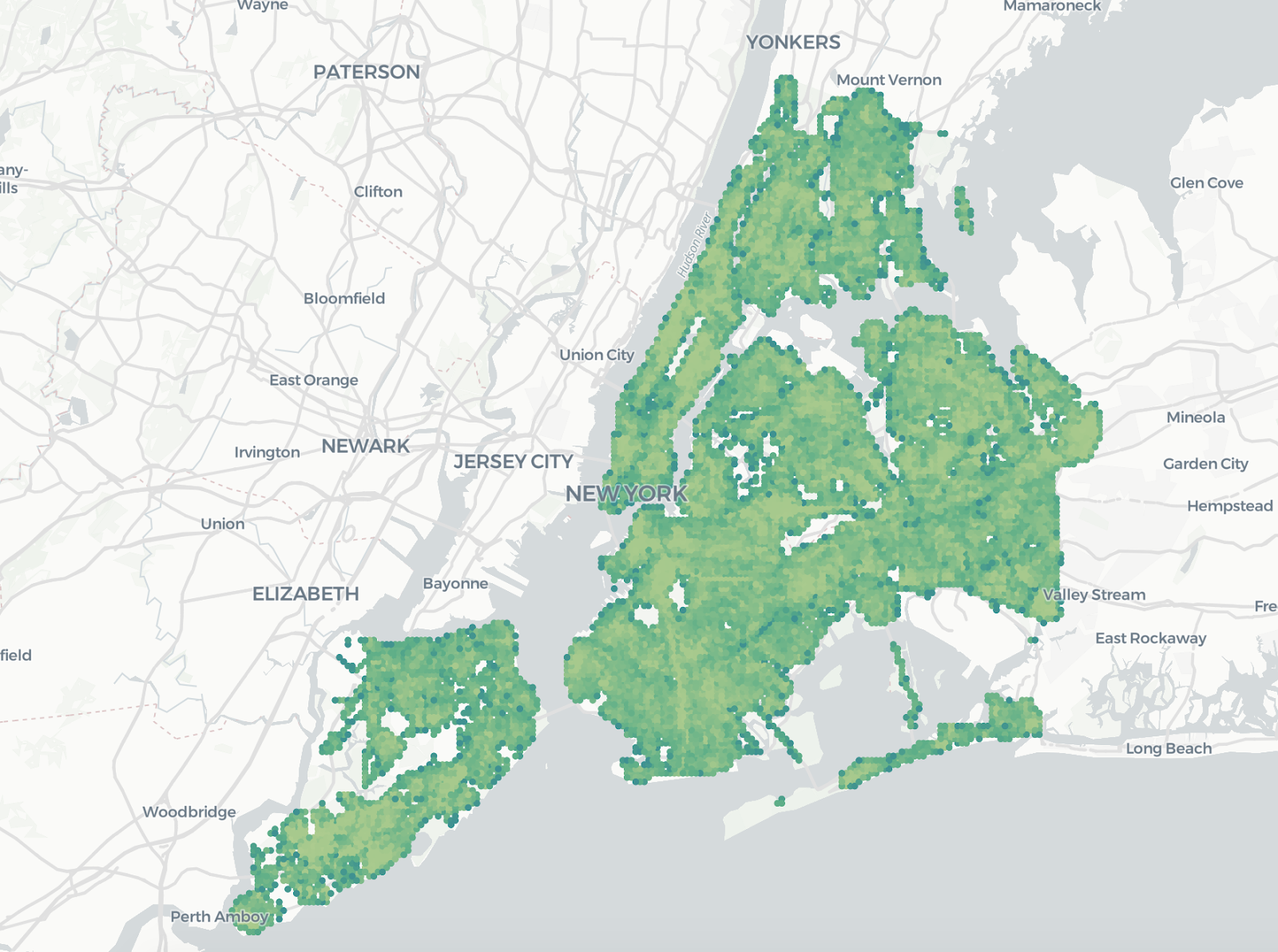
Congrats! You have created your first tileset!
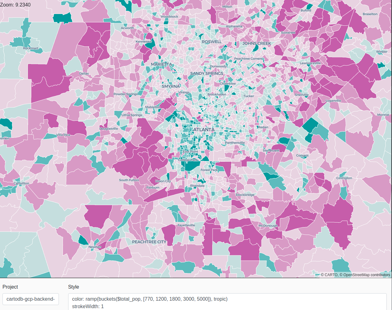
US census blocks (CreateSimpleTileset)
In this example, we want to visualize the US block groups. As those are polygons, we don't want to aggregate them and instead we use the CreateSimpleTileset procedure. To be able to style the visualization, we want to keep 2 properties from the original datasource: a unique identifier (geoid) and the population on those blocks (total_pop).
CALL cartobq.tiler.CreateSimpleTileset(
--SQL to use as the source (uses geom as the name for the geography)
'''
(
  SELECT
    d.geoid,
    d.total_pop,
    g.geom
  FROM `carto-do-public-data.usa_acs.demographics_sociodemographics_usa_blockgroup_2015_5yrs_20142018` d
  JOIN `carto-do-public-data.carto.geography_usa_blockgroup_2015` g
    ON d.geoid = g.geoid
) _input
''',

--Name and location where the Tileset will be stored.
  '`MYORGANIZATIONNAME.MYDATASETID.usa_blockgroup_population`',

--Options on how to generate the Tileset
  '''{
      "zoom_max": 12,
      "max_tile_size_kb": 3072,
      "properties":{
          "geoid": "String",
          "total_pop": "Number"
       }
 }''');
Now that the tileset is generated, you could make it public following the same steps as before and visualize it on the following URL:
https://viewer.carto.com/user/YOURCARTOUSERNAME/bigquery?data=ORGANIZATIONNAME.DATASETID.usa_blockgroup_population&color_by_value=total_pop
As we have mentioned before, we currently provide 2 procedures to tilify a dataset: CreateSimpleTileset and CreatePointAggregationTileset, the first to visualize features individually and the latter to generate aggregated point visualizations.
They are available in the US region under the dataset cartobq.tiler and the EU region under cartobq.tiler_eu (e.g. cartobq.tiler_eu.CreateSimpleTileset).
Both procedures receive 3 parameters (STRING) as input: the source table name or query, the target table and a JSON with other options.
Source table
The first argument is the source table. It can either be a quoted qualified table name or a full query contained by parentheses. Some examples:
`cartodb-gcp-backend-data-team.rmr_tests.points100`(Select * FROM `cartodb-gcp-backend-data-team.rmr_tests.points`)
To avoid issues in the process when building the queries that will be executed internally against BigQuery, it is highly recommended to use raw strings when passing long queries that might contain special characters. For example:
R'''
(
    SELECT
        ST_CENTROID(geometry) as geom
    FROM `bigquery-public-data.geo_openstreetmap.planet_features`
    WHERE
        'building' IN (SELECT key FROM UNNEST(all_tags)) AND
        geometry IS NOT NULL
)
'''
Target table
The second argument defines where the resulting tileset will be stored:
- It must be in the form
`projectID.dataset.tablename`. - The projectID can be omitted (in which case the default one will be used).
- The dataset must exist and the caller needs to have permissions to create a new table on it.
Options
The third and last parameter are the options. It is a string containing a valid JSON with the different options. The current list:
R'''
{
    "geom_column": "geom",

    "zoom_min": 0,
    "zoom_max": 0,
    "zoom_step": 1,

    "tile_extent": 4096,
    "tile_buffer": 0,

    "max_tile_size_kb": 1024,
    "max_tile_size_strategy": "return_null",
    "max_tile_features": 10000,
    "tile_feature_order": "total_pop DESC",

    "target_partitions": 4000,
    "target_tilestats" : true,

-------------------------------------------
-- ONLY IN CreatePointAggregationTileset --
-------------------------------------------
        "type": "quadkey",
        "resolution": 7,
        "placement": "cell-centroid",

        "properties": {
            "aggregated_total": {
                "formula":"count(*)",
                "type":"Number"
            }
        },
        "single_point_properties": {
            "accuracy":"Number"
        }

-------------------------------------------
------- ONLY IN CreateSimpleTileset -------
-------------------------------------------
        "drop_duplicates": true,
        "properties": {
            "geoid": "String",
            "total_pop": "Number"
        }
}
'''
Source table options
geom_column
Default: "geom".
A STRING that marks the name of the geography column that will be used. It must be of type GEOGRAPHY. In
Zoom level options
zoom_min
Default: 0.
A NUMBER that defines the minimum zoom level for tiles. Any zoom level under this level won't be generated.
zoom_max
Default: 0.
A NUMBER that defines the minimum zoom level for tiles. Any zoom level over this level won't be generated.
zoom_step
Default: 1.
A NUMBER that defines the zoom level step. Only the zoom levels that match zoom_min + zoom_step * N, with N being a positive integer will be generated. For example, with { zoom_min: 10, zoom_max: 15, zoom_step : 2 } only the tiles in zoom levels [10, 12, 14] will be generated.
Target options
target_partitions
Default: 4000. Max: 4000.
A NUMBER that defines the maximum amount of partitions to be used in the target table.
The partition system, which uses a column named carto_partition, divides the available partitions first by zoom level and spatial locality to minimize the cost of tile read requests in web maps. Beware that this does not necessarily mean that all the partitions will be used, as sparse dataset will leave some of these partitions unused.
If you are using BigQuery BI Engine consider that it supports a maximum of 500 partitions per table.
target_tilestats
Default: true. Available since version 6.
A BOOLEAN to determine whether to include statistics of the properties in the metadata. This statistics are based on mapbox-tilestats and depend on the property type:
- Number: MIN, MAX, AVG, SUM and quantiles (from 3 to 20 breaks).
- String / Boolean: List of the top 10 most common values and their count.
Note that for aggregation tilesets, these statistics refer to the cells at the maximum zoom generated. In simple tilesets, they are based on the source data.
MVT options
tile_extent
Default: 4096.
A NUMBER defining the extent of the tile in integer coordinates as defined by the MVT spec.
tile_buffer
Default: 16 (0 in aggregation). Available since version 6.
A NUMBER defining the additional buffer added around the tiles in extent units, which is useful to facilitate geometry stitching across tiles in the renderers. In aggregation tilesets, this property is currently not available and always 0 as no geometries go across tile boundaries.
max_tile_size_kb
Default: 1024. Available since version 5.
A NUMBER defining setting the approximate max size for a tile.
max_tile_size_strategy
Default: "return_null" in aggregation, "throw_error" in simple tilesets. Available since version 5.
Determines what to do when the maximum size of a tile is reached while it is still processing data. There are 3 options available:
"return_null": The process will return a NULL buffer. This might appear as empty in the map."throw_error": The process will throw an error cancelling the aggregation, so no tiles or table will be generated."drop_features": The process will stop processing more data and return what it has already processed, ignoring the rest. This could lead to holes in the map.
max_tile_features
Default: 0 (disabled) Available since version 7.
A NUMBER defining setting the max number of features a tile might contain.
This limit is applied before max_tile_size_kb; the tiler will first drop as many features as needed to keep this amount, and then continue with the size limits (if required).
To configure in which order are features kept, use in conjunction with tile_feature_order.
tile_feature_order
Default: "" (Disabled) Available since version 7.
A STRING defining the order in which properties are added to a tile. This expects the SQL ORDER BY keyword definition, such as "aggregated_total DESC", the "ORDER BY" part isn't necessary.
Note that in aggregation tilesets you can only use columns defined as properties, but in simple feature tilesets you can use any source column no matter if it's included in the tile as property or not.
This is an expensive operation, so it's recommended to only use it when necessary.
drop_duplicates
Default: false Available since version 7.
A BOOLEAN to drop duplicate features in a tile. This will drop only exact matches (both the geometry and the properties are exactly equal).
As this requires sorting the properties, which is expensive, it should only be used when necessary.
Properties
Default: {}
A JSON object that defines the extra properties that will be included associated to each cell feature. Each property is defined by its name and type (Number, Boolean or String). In aggregation tilesets you also need to define which formula to use to generate the properties from all the values of the points that fall under the cell.
[CreatePointAggregationTileset]: Properties
When aggregating points we have 2 kinds of properties, the main ones "properties" are the result of an aggregate function and "single_point_properties" are properties that are only available when there is only a single point in the cell, so they are columns from the source data points themselves, not an aggregation.
"properties": {
    "new_column_name": {
        "formula":"count(*)",
        "type":"Number"
    },
    "most_common_ethnicity": {
        "formula":"APPROX_TOP_COUNT(ethnicity, 1)[OFFSET(0)].value",
        "type":"String"
    },
    "has_other_ethnicities":
        "formula":"countif(ethnicity = 'other_race') > 0",
        "type":"Boolean"
    }
},
"single_point_properties": {
    "name":"String",
    "address":"String"
}"new_column_name": The name of the new property. SHOULD not be repeated."formula": Any formula that uses an aggregate function supported by BigQuery and returns the expected type."type": The resulting aggregation type. The type MUST be EXACTLY the string "Number", "Boolean", or "String".
In the example above, for all features we would get a property "new_column_name" with the number of points that fall in it, the "most_common_ethnicity" of those rows and whether there are points whose ethnicity value matches one specific value ("has_other_ethnicities"). In addition to this, when there is only one point that belongs to this property (and only in that case) we will also get the column values from the source data: "name" and "address".
[CreateSimpleTileset]: Properties
In Simple Tilesets, the properties are defined by the source data itself:
"properties": {
    "source_column_name": "Number",
    "source_column_name_2": "String"
    ...
}
In this case the API is simpler as you only have to write the name of the column (as defined in the source query or table) and its type. It doesn't support any extra transformations or formulae since those can be applied to the source query directly.
Spatial aggregation options (CreatePointAggregationTileset)
These options define how the points are aggregated spatially.
type
Default: "quadkey".
A STRING defining what kind of spatial aggregation is to be used. Currently only quadkey is supported.
resolution
Default: 6.
A NUMBER that specifies the resolution of the spatial aggregation.
For quadkey the aggregation for zoom z is done at z + resolution level. For example, with resolution 6, the z0 tile will be divided in cells that match the z6 tiles, or the cells contained in the z10 tile will be the boundaries of the z16 tiles within them. In other words, each tile is subdivided into 4^resolution cells.
Note that adding more granularity necessarily means heavier tiles which take longer to be transmitted and processed in the final client, and you are more likely to hit the internal memory limits.
placement
Default: "cell-centroid".
A STRING that defines what type of geometry will be used for the cells generated in the aggregation.
For a quadkey aggregation, there are currently 4 options:
"cell-centroid": Each feature will be defined as the centroid of the cell, that is, all points that are aggregated together into the cell will be represented in the tile by a single point."cell": Each feature will be defined as the whole cell, thus the final representation in the tile will be a polygon. This gives more precise coordinates but takes more space in the tile and requires more CPU to process it in the renderer."features-any": The point representing a feature will be any random point from the source data, that is, if 10 points fall inside a cell it will use the location of one of them to represent the cell itself."features-centroid": The feature will be defined as the centroid (point) of the points that fall into the cell. Note that this only takes into account the points aggregated under a cell, and not the cell shape (as "cell-centroid" does).
We provide a Python Command Line tool called carto-bq-tiler. Think of it as a supplement to the bq command line tool provided by Google, but with some specific functionality to work with Tilesets. It allows you to:
- Create, list, delete, and manage Tilesets in your BigQuery project
- Visualize privately, using your authentication, your Tilesets
- Upload Tilesets generated using other tools in MBTiles format
- Download a tileset from BigQuery into a set of vector files or a MBTiles file to host your Tilesets somewhere else
Installing carto-bq-tiler
You need to have the Google bq command line tool already installed and working. So check if this command works for you:
bq query "SELECT 1"
If you get something like
You are good to go and you should install carto-bq-tiler like this:
pip3 install carto-bq-tiler
And to check that the tool is working just do:
carto-bq-tiler --help
List your Tilesets
List the Tilesets in your Google Cloud project with:
carto-bq-tiler list
Upload a tileset
You can upload MBTiles files that contain tiles as MVT. The only constraint is that the features must have an id integer property.
carto-bq-tiler load MBTILES_PATH TILESET_NAME
TILESET_NAME is the tileset destination in BigQuery, and it's composed by the dataset and the table as dataset.table.
Delete a tileset
You can simply delete a dataset from BigQuery with:
carto-bq-tileset remove TILESET_NAME
Export a tileset
Tilesets can be exported to your computer in two formats:
- MBTiles files:
carto-bq-tiler export-mbtiles TILESET_NAME
- Directory tree:
carto-bq-tiler export-tiles TILESET_NAME
View a tileset
Tilesets can be viewed and explored in multiple ways:
- A downloaded directory tree:
carto-bq-tiler view-local TILESET_DIRECTORY
- A tileset in BigQuery:
carto-bq-tiler view TILESET_NAME
- A tileset in BigQuery in comparative mode:
carto-bq-tiler view TILESET_NAME -c
- An empty viewer:
carto-bq-tiler view -e
You can also modify the port of the viewer with the --port option.
Authentication
carto-bq-tiler uses the credentials created by the bq command line tool, and it will use the default project configured for it. If you want to use another project you can use the -p (--project) option, like for listing the tilests:
carto-bq-tiler -p PROJECT list
Also, if you have a service account JSON file you can use it instead with -c (--credentials):
carto-bq-tiler -c CREDENTIALS_JSON_PATH list
You can visualize your tilesets in different ways, but overall any tool that supports vector tiles on the MVT format should be good. Here are a few options.
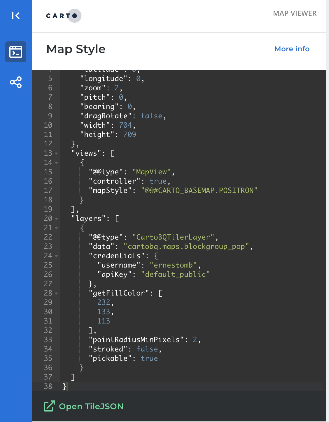
The online viewer
We have created an online viewer that allows you to visualize your tilesets as well as playing with the cartography and style to explore your data. It uses deck.gl declarative style with a set of helper functions that work over the CARTO layers.
In order to "publish" a tileset, you need to provide "BigQuery Data Viewer" permissions in BigQuery. There are several different options:
- Make the tileset available to anyone on the internet using the
allUsersmember. - Make the tileset available to anyone authenticated with a Google account using the
allAuthenticatedUsersmember. - Make the tileset available only to CARTO Maps API v2 beta Service Account:
maps-api-v2@avid-wavelet-844.iam.gserviceaccount.com
Once you do that you can start retrieving tiles directly from BigQuery without authentication. Here are a few URLs you will need to know:
https://viewer.carto.com/user/USERNAME/bigquery?data=PROJECT.DATASET.tileset
Click the link above to see an example.
Additionally, using the color_by_value=property parameter in the viewer's URL, you can have a color ramp automatically applied to your visualization.
Opening a TileJSON URL in the browser, you will find some statistics calculated over the data attribute included in the tileset:
{
        "attribute": "total_pop",
        "type": "Number",
        "min": 0,
        "max": 55407,
        "avg": 1484.9313442617063,
        "sum": 326289904,
        "quantiles": [
          {
            "3": [
              1002,
              1594
            ]
          },
          {
            "4": [
              897,
              1270,
              1822
            ]
          },
          (...)
The quantiles object contains the breaks for different quantiles classifications, that you can use in your visualization, copying and pasting the breaks from the TileJSON to the styling section:
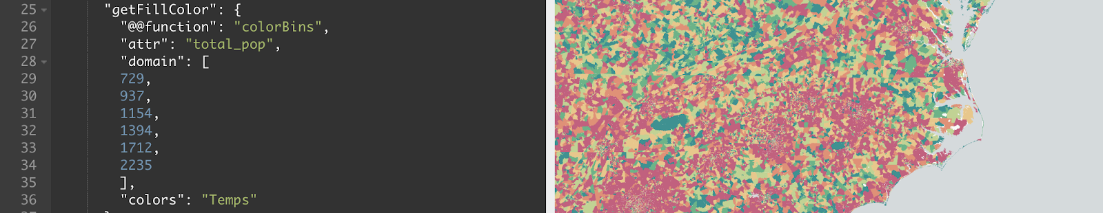
Declarative styling with deck.gl
The online viewer works with deck.gl and the visualization's cartographic style can be defined with deck.gl declarative language.
Here is a more complete reference (although still a work in progress) of all the keys that can be used to style a CARTO layer.
Here is also the CARTO styling helpers for deck.gl reference, for different color ramp methods.
Other options
You could always just retrieve the tiles and use them with any other vector tiles client.
Check out the next section on QGIS to learn how to get the TileJSON and then request tiles directly.
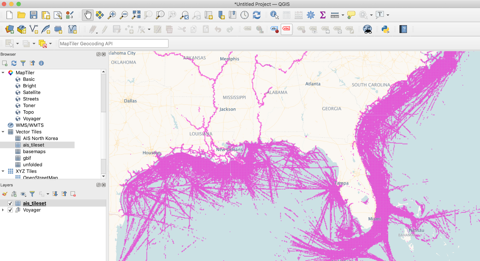
Using QGIS
QGIS provides support for Vector Tiles since version 3.14.
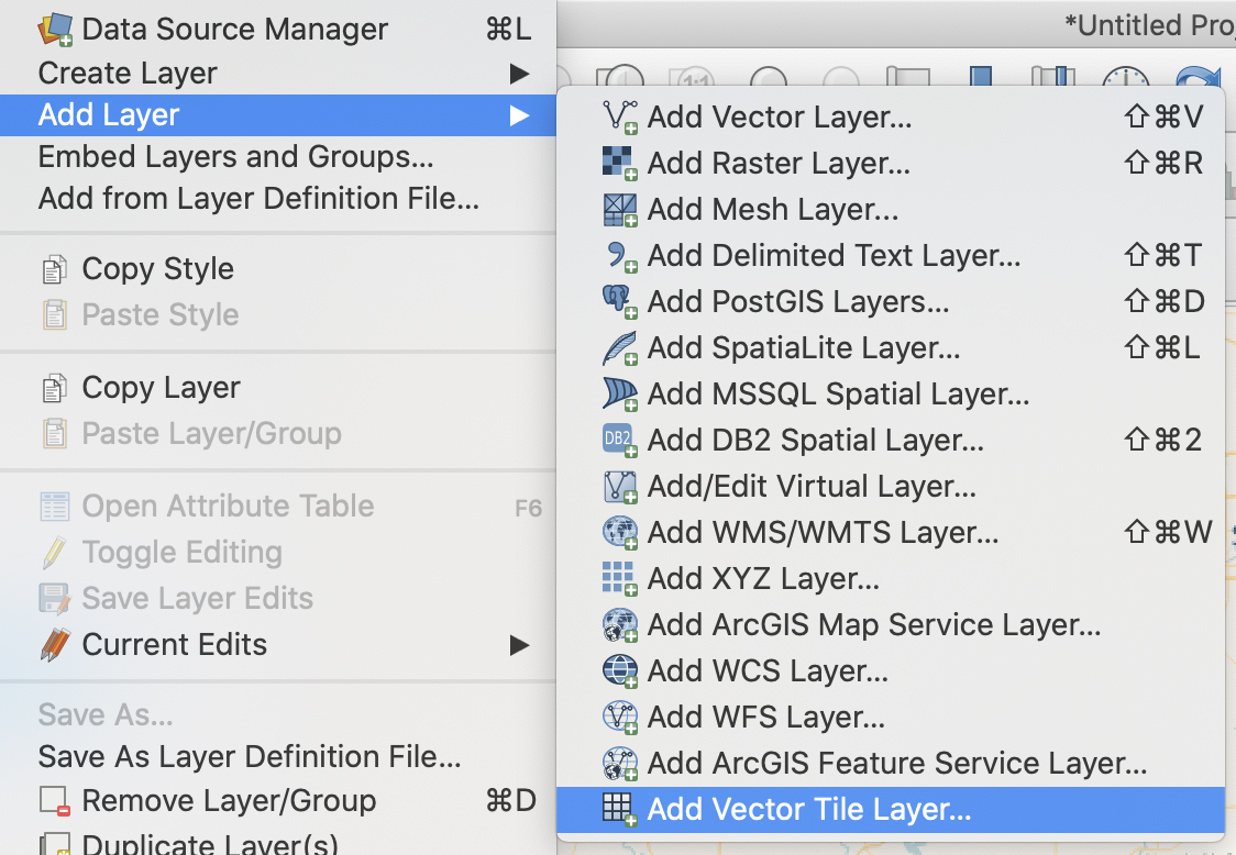
You will be prompted to create a connection:
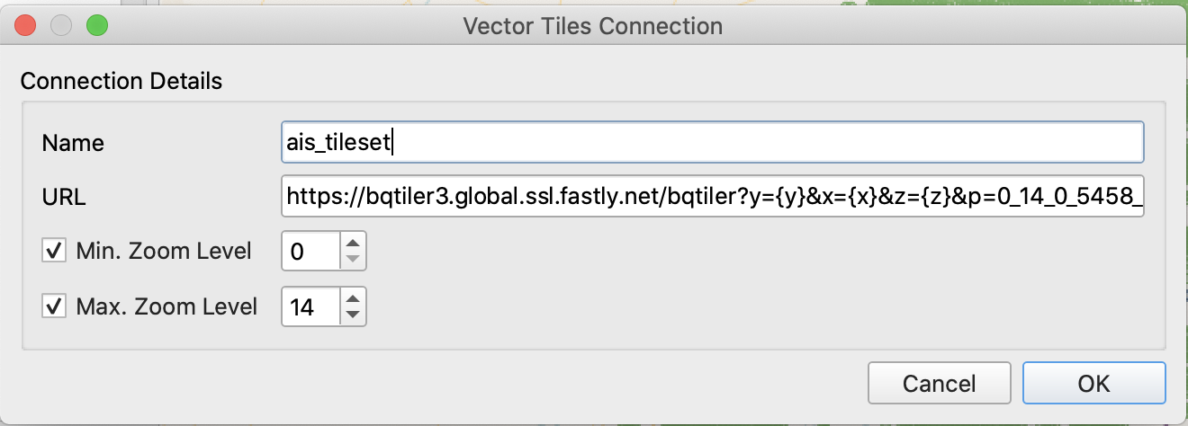
Name: name of the layer on the QGIS layers panel.
URL: You can get a TileJSON URL by clicking on the "Open TileJSON" button in the Map Style section of the online viewer:
Or with a request to the Maps API with the following structure:
When you open that URL you will see a JSON on it that contains the URL from where to retrieve the tile Template that you need to enter on the URL field. For example:
https://maps-api-v2.us.carto.com/user/ernestomb/bigquery/tileset/{z}/{x}/{y}?source=cartobq.maps.blockgroup_pop&partition=0_14_38_16374_3475_7365_4000_1&format=mvt&cache=1603812883827&api_key=default_publicOnce you enter this information, the layer will appear:
Using deck.gl and Google Maps
Here are a couple of examples using deck.gl with Google Maps basemaps
- https://bl.ocks.org/jatorre/02331191ac0ea94a961073371529d029
- https://bl.ocks.org/jatorre/29d7ec68d39f18eb534c01e9e0326d76
Aggregation: OSM buildings
We want to make use of the OSM BigQuery Dataset to visualize all the features tagged as ‘building' them. Since the dataset has different types of geometries for the buildings, It uses ST_CENTROID to ensure they all are points.
The extra column, aggregated_total, is adding a count for the number of buildings that are aggregated into a cell, which in this case are quadkeys made of z + resolution tiles, that is, each tile will be subdivided into 4^7 (16384) cells.
CALL cartobq.tiler.CreatePointAggregationTileset(
  R'''(
        SELECT
            ST_CENTROID(geometry) as geom
        FROM `bigquery-public-data.geo_openstreetmap.planet_features`
        WHERE 'building' IN (SELECT key FROM UNNEST(all_tags)) AND
               geometry IS NOT NULL
    )''',
  '`your-project.your-dataset.osm_buildings_14_7`',
  R'''
    {
      "zoom_min": 0,
      "zoom_max": 14,
      "type": "quadkey",
      "resolution": 7,
      "placement": "cell-centroid",
      "properties":{
        "aggregated_total": {
          "formula":"count(*)",
          "type":"Number"
        }
      }
    }
  ''');
This process will take the over 300M buildings in the source table, aggregate them into cells and generate a table containing more than 4M tiles around the world.
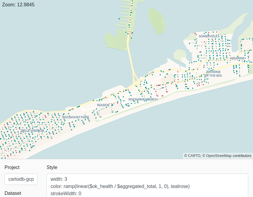
Aggregation: NYC happy little trees
In this case we want to visualize the tree census of NYC. Since the table doesn't have a geography column, we are going to create it on the fly using the latitude and longitude columns.
We also want to have access to the status and health of each aggregated cell, so we add some extra properties around that. Finally, as it is a more localized dataset, we want to generate higher zoom levels (16) and when we see individual points we want access to both their official id and their address.
CALL cartobq.tiler.CreatePointAggregationTileset(
  R'''(
        SELECT
            ST_GEOGPOINT(longitude, latitude) as geom,
            status, health, tree_id, address
        FROM `bigquery-public-data.new_york_trees.tree_census_2015`
    )''',
  '`your-project.your-dataset.test_tilesets.nyc_trees_16_7`',
  R'''
    {
      "zoom_max": 16,
      "type": "quadkey",
      "resolution": 7,
      "placement": "features-centroid",
      "properties":{
        "aggregated_total": {
          "formula": "count(status)",
          "type": "Number"
        },
        "alive_total": {
          "formula": "countif(status = 'Alive')",
          "type": "Number"
        },
        "ok_health": {
          "formula": "countif(health = 'Good' OR health = 'Fair')",
          "type": "Number"
        }
      },
      "single_point_properties": {
           "tree_id": "Number",
           "address": "String"
      }
    }
  ''');
Then we can style our visualization using the properties that we have added:
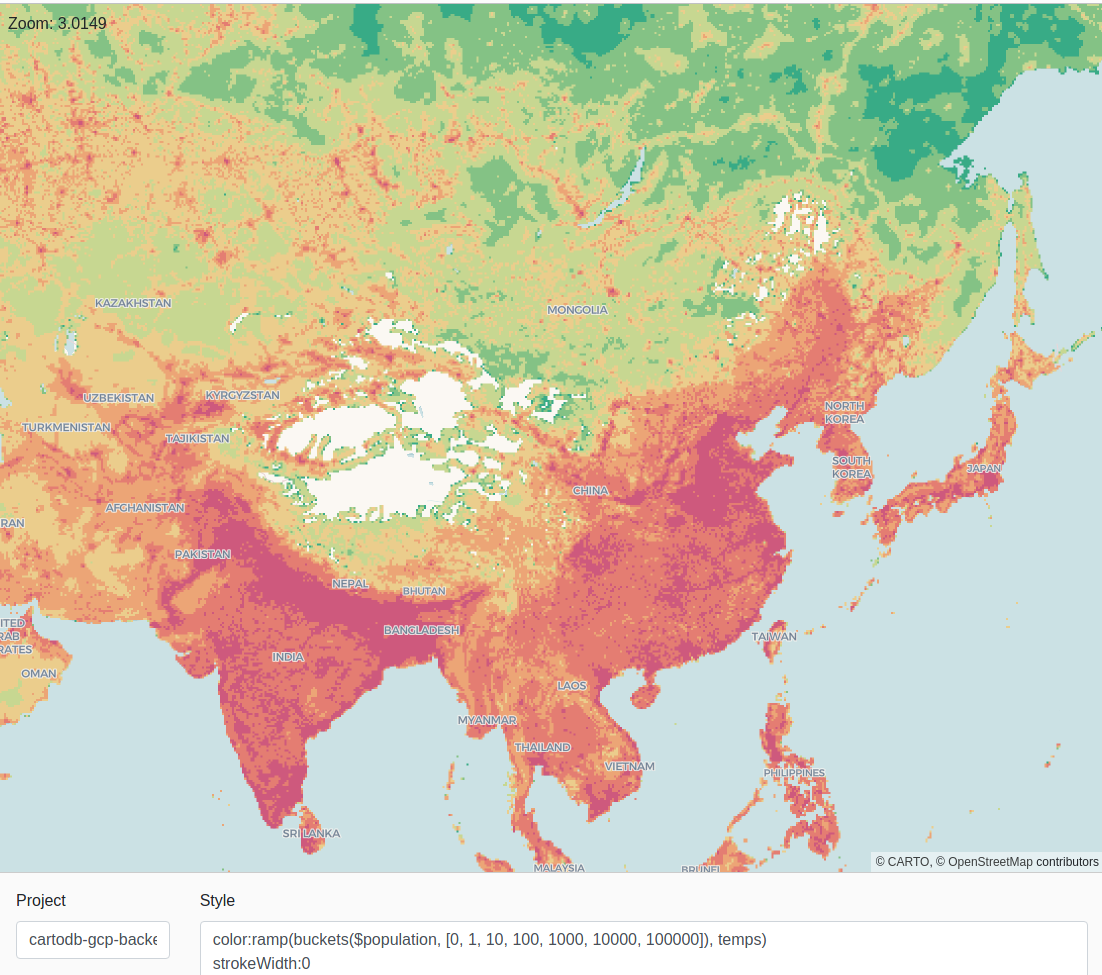
Aggregation: 2020 world population
For this example we are going to use CARTO's public data observatory to visualize the 2020 world population. In the first case we are going to use the already aggregated 1km*1km grids:
CALL cartobq.tiler.CreatePointAggregationTileset(
  R'''(
        SELECT ST_Centroid(b.geom) as geom, population
        FROM
          `carto-do-public-data.worldpop.demographics_population_glo_grid1km_v1_yearly_2020` a
        INNER JOIN
          `carto-do-public-data.worldpop.geography_glo_grid1km_v1` b
        ON (a.geoid = b.geoid)
    )''',
  '`your-project.your-dataset.wpop_2020_1km_cell`',
  R'''
    {
      "zoom_max": 6,
      "type": "quadkey",
      "resolution": 7,
      "placement": "cell",
      "columns":{
        "population": {
          "formula": "sum(population)",
          "type": "Number"
        }
      }
    }
  ''');
Note that since this comes from already aggregated areas, it doesn't make sense to go to high zoom levels, but visualize the data at country scale.
Lines: Natural Earth roads
Using also CARTO's public data observatory we are going to visualize
In the first case we are going to use the already aggregated 1km*1km grids:
CALL cartobq.tiler.CreateSimpleTileset(
  R'''
(
  SELECT geom, type
  FROM `carto-do-public-data.natural_earth.geography_glo_roads_410`
) _input
  ''',
  R'''`cartobq.maps.natural_earth_roads`''',
  R'''
  {
      "zoom_min": 0,
      "zoom_max": 10,
      "max_tile_size_kb": 3072,
      "properties":{
          "type": "String"
       }
  }'''
);
The result is a worldwide map with the requested tiles, including the type of each road.
Polygons: US block groups
In the same exact way we generated the tileset including lines, we can generate a tileset that uses polygons as its source geography type.
CALL cartobq.tiler.CreateSimpleTileset(
  R'''
(
  SELECT
    d.geoid,
    d.total_pop,
    g.geom
  FROM `carto-do-public-data.usa_acs.demographics_sociodemographics_usa_blockgroup_2015_5yrs_20142018` d
  JOIN `carto-do-public-data.carto.geography_usa_blockgroup_2015` g
    ON d.geoid = g.geoid
) _input
  ''',
  R'''`cartobq.maps.blockgroup_pop`''',
  R'''
  {
      "zoom_min": 0,
      "zoom_max": 14,
      "max_tile_size_kb": 3072,
      "properties":{
          "geoid": "String",
          "total_pop": "Number"
       }
  }'''
);
We can style the result based on the properties added (total_pop) as shown in the initial example or visualize it in the default UI service.
- It is currently not possible to rewrite the target table if it already exists.
- In CreatePointAggregationTileset The
idfield of all the features israndomso, although extremely unlikely, there might be duplicates. CreateSimpleTileset doesn't include anidso you might want to include your own identifying property. - Sparse dataset (or datasets with outliers) will have a suboptimal partition system, as most of the assigned partitions will be empty.
- There are internal BigQuery limits that the tiler can't overcome: The amount of data passed as input for a single tile shouldn't be bigger than 100MB, and the max size of the resulting single tile shouldn't be bigger than 5MB.
For example, if you have a dataset with duplicate geographies and try to include them all, you can reach these limits and get errors like: Resources exceeded during query execution: The query could not be executed in the allotted memory. Another example of this is if you try to visualize a point dataset using CreateSimpleTileset at a low zoom level, since that will try to put all the points into the tile. - CreateSimpleTileset does not support mixing geometry types in the same tileset. This isn't really a BQTiler limitation, but an issue with most of the renderers being unable to work different geometry types in the same layer.
2020-12-03 - Internal version: 7
- Both procedures (CreateSimpleTileset and CreatePointAggregationTileset):
- Add the
"max_tile_features"option to limit the amount of features a tile might contain (independently from its size). Best when coupled with"tile_feature_order". - Add the
"tile_feature_order"option to decide the order in which features are added into the tile. - Add the internal option
"force_parallelism". - Change quantile tilestats from an array of objects to an object with arrays as properties, matching MAPS API v2.
- CreateSimpleTileset:
- Add support for geometry collections (extracts the higher order dimension).
- Add the
"drop_duplicates"option to drop exact duplicates. - CreatePointAggregationTileset:
- Add new placement options.
"features-any"returns any (random) point from the source data as the value for the cell."features-centroid"returns the centroid of the points aggregated under the cell. Note that this only takes into account the points aggregated under a cell, and not the cell shape (as"cell-centroid"does).- Add the
"single_point_properties"option, which are properties from the source dataset/table that are only included in the feature when there is a single point inside the cell.
2020-10-27 - Internal version: 6
Fourth public release for beta testers:
- CreateSimpleTileset: New procedure to tilify individual features (no aggregation)
- ST_PointAggregationAsMVT renamed as CreatePointAggregationTileset:
- API changes in the declaration of properties.
"columns"renamed to"properties"."function"and"column"replaced by"formula".- Added target_tilestats option to add statistics about the properties in the metadata.
- Changed the numeric values of the metadata (such as maxzoom) to be stored as integers (they used to be saved as strings).
- Version 0.1.5 of the console client.
2020-09-10 - Internal version: 5
Third public release for beta testers.
- ST_PointAggregationAsMVT:
- Changed the MVT feature id from 0 to a random integer [0..2^53)
- 2 new options (max_tile_size_kb, max_tile_size_strategy) to control the maximum size of tiles and what to do when the limit is reached.
- Fix a bug in the metadata when the input query contains backslashes.
- The whole process has been simplified internally, improving the error management and halving the base time (before the main query).
- Now available in the EU processing region (cartobq.tiler_eu).
- Add a Version() function, useful to test if permissions are working.
- Fix a bug in ST_AsMVT where a property with NULL value would be included in the MVT as the boolean value "false". Following the MVT spec, now it won't be included.
- Released version 0.1.4 of the console client.
2020-07-14 - Internal version: 4
Second alpha release for beta testers.
- Moved the metadata from the table description to tile -1/NULL/NULL
- Applied a couple of changes in the default renderer to reduce the number of tile requests.
2020-07-01 - Internal version: 3
First alpha release for beta testers.
- Partition version: 1
MVT
The MVT format is a space-efficient encoding format for tiled geographic vector data. It is an open standard which has many implementations both for generators (such us Mapnik or PostGIS) or clients (MapboxGL, CARTO VL, deck.gl...).
They were designed with dynamic map styling on mind, so they tend to be really small, but beware of adding too many properties associated with a geospatial feature since that will lead to much bigger tiles and slower load times. To avoid bloated tiles, it is recommended to only include the data needed to style the map, and set up a different endpoint to access occasional data related to the properties.
Now in bold letters: You should not treat MVT as a way to extract data out of BigQuery. There are way better formats to do so. If you find yourself adding more than 4-5 data columns per feature (aside from the geometry itself), you should consider setting up a different endpoint to access those properties.
We have developed an internal function with an equivalent behaviour to Postgis' ST_AsMVT, that is, a function that receives data that is part of a tile, processes it and generates the final buffer that is the MVT.
As defined by the specification, this tile is encoded as a protobuf. To reduce both the storage and transmission costs, the buffer is compressed using gzip (any modern browser has built-in support for it). Lastly, due to limitations in BigQuery APIs, the final result is encoded using Base64 which is what we end up storing. To summarize:
data column := base64(gzip(protobuf(geometries + properties)))Webmercator tiles
In case you are not familiar with the term tile in the context of a web map, we would recommend you to give this Wikipedia article a quick read. There are several concepts that have a tight relationship with this:
- Zoom level. We start mapping at zoom 0, with a single tile that covers the whole world. The next zoom level, 1, is defined as a subdivision of this original tile. Each of the 2 axes (x and y) is divided by half, which gives us 4 tiles: x can be 0 or 1, y can be 0 or 1. So we get 1/0/0, 1/0/1, 1/1/0 and 1/1/1 as the 4 possible tiles at zoom level 1.
The next zoom level, 2, will be formed by dividing each of those tiles again by half, so we get 2/0/0 .. 2/3/3 for a total of 16 tiles. And we could continue this process for as long as we wanted to.
The tiles we generate follow the z/x/y convention.
- Projection. Sadly for us, the world isn't flat, which means that to represent it on a flat surface, like a 2D web map, you need to project the different Earth points into the final surface. There are many different so-called projections, and we are using the Web Mercator projection (EPSG:3857) which is the most common one used in web mapping.
- Screen size. When using raster images (such as .pngs) to render a tile in the screen, it's straightforward to decide how much screen space to assign to each tile as they have a fixed size (typically 256x256 pixels), so unless you are using decimal zoom level the easiest way to handle it is to place as you get it. On the other hand, vector images don't have any predefined pixel size. This does not mean that the MVTs weren't generated with a pixel size in mind (again for integer numbers), and in the case of the BQ Tiler this value is 512. That is, the tile 1/0/1 is meant to take 512x512 pixels when represented at zoom 1.0. Bear in mind that this is just a recommendation and you can still use as many pixels as you want per tile.
Visualization
We provide a service so that you can create and share maps publicly, which reads the data from BigQuery and offers a HTTP endpoint that can be fed to any MVT client. If you want to avoid this and create your own service or create an application that reads directly from BigQuery, we share here the structure of the destination table.
Data structure
All the generated tiles are stored in a single table with the following schema:
Field name | Description |
z | A INT64 value defining the tile zoom level. |
x | A INT64 value defining the horizontal position in the XY scheme. |
y | A INT64 value defining the vertical position in the XY scheme. |
carto_partition | A INT64 value used internally to partition the tileset into equivalent zones so it's cheaper and faster to read from the table to do visualizations. It is generated using the |
data | The MVT tile itself. |
There is also extra metadata information stored in the table (z=-1, x=null, y=null, carto_partition=null) that can be useful for rendering, such as vector_layers which include information about the feature properties, tilestats with information about the values contained in the tiles, or the carto_partition metadata, used to calculate in which partition each tile is placed.
Finally, all tiles will have a label "carto_tileset" : $version. This is used to easily locate all the Tilesets within a project.
Code
There are 2 HTML examples included in the python client (bigquery_viewer.html and bigquery_viewer_compare.html that can be used as reference. They are using CARTO VL to visualize the tile, so there are many options available to style your data.
For example, this changes the color of the data based on using a ramp over the aggregated_total property, using the temps color scheme:
color:ramp(buckets($aggregated_total, [0, 1, 10, 100, 1000, 10000, 100000]), temps)
strokeWidth:0